User:Dwight Landen/sandbox
bla bla what does this look like?
Time-frequency Analysis with the short-time Fourier transform[edit]
Spectral moments[edit]
Resolution issues[edit]
One of the perceived downfalls of the STFT is related or analogous to Heisenberg uncertainty principle, but it is not a direct relationship – see Gabor limit for discussion. The width of the windowing function relates to how the signal is represented; it determines spread or support of the function in the frequency domain. A wide time window results in a narrow frequency range. A narrower time window results in a wide frequency range. These are called narrowband and wideband transforms, respectively. In a more rigorous manner the duration and bandwidth can be defined
- .
Where the bar denotes the mean. It can then be shown that the uncertainty product is
An additional complication arises when considering the discrete STFT. Discrete signals must consider not only the length of the time window but the sample rate. Sample rate will determine the maximum frequency that can be represented without aliasing or Nyquist frequency. Together, a STFT with no overlap and window length will have an uncertainty product of
For a fixed time window, this means that a high sample rate with good time resolution will have a high Nyquist frequency and therefore the points will be spread over a wide range and thus frequency resolution will be poor. A low sample rate will have lower time resolution with a low Nyquist frequency with point spread over a narrow range thus better frequency resolution.

The choice of window functions are many, each with there own purpose. The boundary of the uncertainty principle is reached with a Gaussian window function, as the Gaussian minimizes the Fourier uncertainty principle. [2] This is called the Gabor transform (and with modifications for multiresolution becomes the Morlet wavelet transform). One can consider the STFT for varying window size as a two-dimensional domain (time and frequency), as illustrated in the example below, which can be calculated by varying the window size. However, this is no longer a strictly time–frequency representation – the kernel is not constant over the entire signal.
Example[edit]
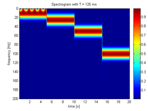
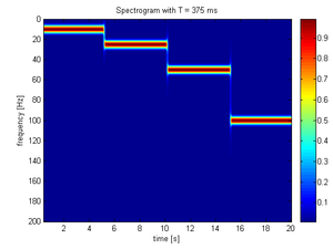
Using the following sample signal that is composed of a set of four sinusoidal waveforms joined together in sequence. Each waveform is only composed of one of four frequencies (10, 25, 50, 100 Hz). The definition of is:
Then it is sampled at 400 Hz. The following spectrograms were produced:
 |
 |
 |
 |
The 25 ms window allows us to identify a precise time at which the signals change but the precise frequencies are difficult to identify. At the other end of the scale, the 1000 ms window allows the frequencies to be precisely seen but the time between frequency changes is blurred.
This is one of the reasons for the creation of the wavelet transform and multiresolution analysis, which can give good time resolution for high-frequency events, and good frequency resolution for low-frequency events, which is the type of analysis well suited for many real signals.
Local Mean Frequency[edit]
It is often then mistaken that the ability to determine the instantaneous frequency in limited by the uncertainty principle. The instantaneous frequency or "local mean frequency" can be very accurately determined and is limited more by the continuity of the instantaneous phase.[3] To understand this the spectral density of the analytic signal must be considered
and
- .
The nth moment (mathematics) of the spectrum is given by
Which can also be expressed in the time domain as
The first moment or "local mean" is
where
- .[3]
and
- .
Substituting the Gaussian window for and using the Taylor expansion of at the midpoint of the sliding window , the expansion is
where are the moments of with the expansion
- .[3]
where is the standard deviation of the Gaussian window. The resulting expansion of the local mean is
Bandwidth[edit]
Optimal Windows[edit]
Continuity and Accuracy Errors[edit]
References[edit]
- ^ a b *Cohen, Leon (1995), Time-frequency Analysis: Theory and Applications, Prentice-Hall
- ^ *Hamming, R.W. (1998), Digital Filters, Courier Dover Publications
- ^ a b c d e *Cohen, L.; Lee, C. (1989), Local Bandwidth and Optimal Window for the Short Time Fourier Transform, Society of Photo-Optical Instrumentation Engineers (SPIE) Conference Series, pp. 402–425


