https://en.wikipedia.org/wiki/Spectral_gap_(physics)
https://en.wikipedia.org/wiki/Duality_gap
+
https://en.wikipedia.org/wiki/Doubly_periodic_function
https://en.wikipedia.org/wiki/Fundamental_pair_of_periods
div
F
=
∇
⋅
F
=
tr
(
J
(
f
)
)
{\displaystyle \operatorname {div} \mathbf {F} =\nabla \cdot \mathbf {F} =\operatorname {tr} (\mathbf {J} (f))}
+
Δ
f
=
∇
2
f
=
∇
⋅
∇
f
=
tr
(
H
(
f
)
)
{\displaystyle \Delta f=\nabla ^{2}f=\nabla \cdot \nabla f=\operatorname {tr} {\big (}H(f){\big )}}
+
+
Group diagrams [ edit ] https://commons.wikimedia.org/wiki/Category:Mathematical_diagrams
https://commons.wikimedia.org/wiki/Category:Commutative_diagrams
https://commons.wikimedia.org/wiki/Category:Group_theory
https://commons.wikimedia.org/wiki/File:Projective-representation-lifting.svg +]
+
+
+
+
+
+
groups: https://en.wikipedia.org/wiki/Bézout's_identity https://en.wikipedia.org/wiki/Chinese_remainder_theorem
https://en.wikipedia.org/wiki/Weierstrass_transform#Generalizations
https://en.wikipedia.org/wiki/Shift_operator
https://en.wikipedia.org/wiki/Operator_(physics)#The_exponential_map
+
π
k
(
x
)
∼
x
(
log
log
x
)
k
−
1
(
k
−
1
)
!
log
x
(
1
)
{\displaystyle \pi _{k}(x)\sim {\frac {x(\log \log x)^{k-1}}{(k-1)!\log x}}\qquad \qquad (1)}
+
π
2
(
x
)
∼
1.32
x
(
log
x
)
2
{\displaystyle \pi _{2}(x)\sim 1.32{\frac {x}{(\log x)^{2}}}}
+
p
n
≈
n
log
n
+
n
(
log
log
n
−
1
)
,
{\displaystyle p_{n}\approx n\log n+n(\log \log n-1),}
∑
n
≤
x
σ
0
(
n
)
≈
x
log
x
+
x
(
2
γ
−
1
)
{\displaystyle \sum _{n\leq x}\sigma _{0}(n)\approx x\log x+x(2\gamma -1)}
lim
n
→
∞
1
log
n
∏
p
≤
n
p
p
−
1
=
e
γ
,
{\displaystyle \lim _{n\to \infty }{\frac {1}{\log n}}\prod _{p\leq n}{\frac {p}{p-1}}=e^{\gamma },}
lim sup
n
→
∞
σ
(
n
)
n
log
log
n
=
e
γ
{\displaystyle \limsup _{n\rightarrow \infty }{\frac {\sigma (n)}{n\,\log \log n}}=e^{\gamma }}
+
+
+
https://en.wikipedia.org/wiki/Chern-Simons_theory#HOMFLY_and_Jones_polynomials
https://en.wikipedia.org/wiki/Weyl_character_formula#The_SU(2)_case
https://en.wikipedia.org/wiki/Representation_theorem
https://en.wikipedia.org/wiki/Vanishing_theorem
https://en.wikipedia.org/wiki/Analytic_torsion
https://en.wikipedia.org/wiki/Crooks_fluctuation_theorem
⟨
A
⟩
=
tr
(
A
ρ
)
{\displaystyle \langle A\rangle =\operatorname {tr} (A\rho )}
+
+
+
+
E
[
exp
(
−
t
X
)
]
=
.
.
.
{\displaystyle \operatorname {E} [\exp(-tX)]=...}
∫
exp
(
−
(
X
−
E
[
X
]
)
2
2
E
[
(
X
−
E
[
X
]
)
2
]
)
=
(
det
(
E
[
(
X
−
E
[
X
]
)
2
)
)
1
2
{\displaystyle \int \exp(-{\frac {(X-\operatorname {E} [X])^{2}}{2\operatorname {E} [(X-\operatorname {E} [X])^{2}]}})=(\operatorname {det} (\operatorname {E} [(X-\operatorname {E} [X])^{2}))^{\frac {1}{2}}}
https://en.wikipedia.org/wiki/Agoh-Giuga_conjecture
https://en.wikipedia.org/wiki/Daniel_da_Silva_(mathematician)
https://en.wikipedia.org/wiki/Euler's_identity#Generalizations
https://en.wikipedia.org/wiki/Crenel_function
https://en.wikipedia.org/wiki/Montgomery's_pair_correlation_conjecture
https://en.wikipedia.org/wiki/Cyclotomic_polynomial
https://proofwiki.org/wiki/Reciprocals_of_Odd_Numbers_adding_to_1
https://en.wikipedia.org/wiki/Chebyshev_function#The_Riemann_hypothesis
https://en.wikipedia.org/wiki/Explicit_formulae_(L-function)#Weil's_Explicit_Formula
https://en.wikipedia.org/wiki/Hilbert–Pólya_conjecture
https://mathoverflow.net/questions/62816/the-guinand-weil-explicit-formula-without-entire-function-theory?rq=1
https://en.wikipedia.org/wiki/Cassini_and_Catalan_identities
https://en.wikipedia.org/wiki/Generating_function
https://en.wikipedia.org/wiki/Table_of_Newtonian_series
ζ
(
1
−
n
,
a
)
=
−
B
n
(
a
)
n
{\displaystyle \zeta (1-n,a)=-{\frac {B_{n}(a)}{n}}\!}
n
≥
1
{\displaystyle n\geq 1\!}
+
ζ
(
2
n
)
=
(
−
1
)
n
+
1
B
2
n
(
2
π
)
2
n
2
(
2
n
)
!
{\displaystyle \zeta (2n)={\frac {(-1)^{n+1}B_{2n}(2\pi )^{2n}}{2(2n)!}}}
ζ
(
−
n
)
=
(
−
1
)
n
B
n
+
1
n
+
1
{\displaystyle \zeta (-n)=(-1)^{n}{\frac {B_{n+1}}{n+1}}}
Hodge duality ->Poincaré duality ->Grothendieck local duality ->Serre duality
kunneth theorem
+
+
[+
https://en.wikipedia.org/wiki/Dedekind_psi_function
https://mathoverflow.net/questions/14083/modular-forms-and-the-riemann-hypothesis
p
(
x
)
=
1
2
π
∫
R
e
i
t
x
P
(
t
)
d
t
=
1
2
π
∫
R
e
i
t
x
φ
X
(
t
)
¯
d
t
.
{\displaystyle p(x)={\frac {1}{2\pi }}\int _{\mathbf {R} }e^{itx}P(t)\,dt={\frac {1}{2\pi }}\int _{\mathbf {R} }e^{itx}{\overline {\varphi _{X}(t)}}\,dt.}
+
+
+
+
f
^
(
x
)
=
1
2
π
∫
−
∞
+
∞
φ
^
(
t
)
ψ
h
(
t
)
e
−
i
t
x
d
t
=
1
2
π
∫
−
∞
+
∞
1
n
∑
j
=
1
n
e
i
t
(
x
j
−
x
)
ψ
(
h
t
)
d
t
=
1
n
h
∑
j
=
1
n
1
2
π
∫
−
∞
+
∞
e
−
i
(
h
t
)
x
−
x
j
h
ψ
(
h
t
)
d
(
h
t
)
=
1
n
h
∑
j
=
1
n
K
(
x
−
x
j
h
)
{\displaystyle {\widehat {f}}(x)={\frac {1}{2\pi }}\int _{-\infty }^{+\infty }{\widehat {\varphi }}(t)\psi _{h}(t)e^{-itx}\,dt={\frac {1}{2\pi }}\int _{-\infty }^{+\infty }{\frac {1}{n}}\sum _{j=1}^{n}e^{it(x_{j}-x)}\psi (ht)\,dt={\frac {1}{nh}}\sum _{j=1}^{n}{\frac {1}{2\pi }}\int _{-\infty }^{+\infty }e^{-i(ht){\frac {x-x_{j}}{h}}}\psi (ht)\,d(ht)={\frac {1}{nh}}\sum _{j=1}^{n}K{\Big (}{\frac {x-x_{j}}{h}}{\Big )}}
φ
Z
n
(
t
)
=
(
φ
Y
1
(
t
n
)
)
n
=
(
e
−
1
2
(
t
n
)
2
)
n
=
e
−
t
2
2
{\displaystyle \varphi _{Z_{n}}(t)=(\varphi _{Y_{1}}({\frac {t}{\sqrt {n}}}))^{n}=(e^{-{\frac {1}{2}}({\frac {t}{\sqrt {n}}})^{2}})^{n}=e^{-{\frac {t^{2}}{2}}}}
K
~
(
p
;
T
)
=
G
~
ε
(
p
)
T
/
ε
=
(
e
−
1
2
(
ε
p
)
2
)
T
/
ε
=
e
−
T
p
2
2
{\displaystyle {\tilde {K}}(p;T)={\tilde {G}}_{\varepsilon }(p)^{T/\varepsilon }=(e^{-{\frac {1}{2}}({\sqrt {\varepsilon }}p)^{2}})^{T/\varepsilon }=e^{-{\frac {Tp^{2}}{2}}}}
ψ
t
(
y
)
=
∫
ψ
0
(
x
)
K
(
x
−
y
;
t
)
d
x
=
∫
ψ
0
(
x
)
∫
x
(
0
)
=
x
x
(
t
)
=
y
e
i
S
D
x
,
{\displaystyle \psi _{t}(y)=\int \psi _{0}(x)K(x-y;t)\,dx=\int \psi _{0}(x)\int _{x(0)=x}^{x(t)=y}e^{iS}\,Dx,}
K
(
x
,
y
;
T
)
=
∫
x
(
0
)
=
x
x
(
T
)
=
y
∏
t
exp
(
−
1
2
(
x
(
t
+
ε
)
−
x
(
t
)
ε
)
2
ε
)
D
x
,
{\displaystyle K(x,y;T)=\int _{x(0)=x}^{x(T)=y}\prod _{t}\exp \left(-{\tfrac {1}{2}}\left({\frac {x(t+\varepsilon )-x(t)}{\varepsilon }}\right)^{2}\varepsilon \right)\,Dx,}
"Index theory" [ edit ]
∑
i
(
−
1
)
i
Tr
(
Frob
,
H
c
i
(
X
,
Q
ℓ
)
)
=
|
X
(
F
q
)
|
{\displaystyle \sum _{i}(-1)^{i}{\text{Tr}}({\text{Frob}},H_{c}^{i}(X,{\bf {{Q}_{\ell }))=|X({\bf {F}}_{q})|}}}
∑
i
(
−
1
)
i
T
r
(
f
∗
|
H
k
(
X
,
Q
)
)
=
∑
x
∈
F
i
x
(
f
)
i
n
d
e
x
x
f
{\displaystyle \sum _{i}(-1)^{i}\mathrm {Tr} (f_{*}|H_{k}(X,\mathbb {Q} ))=\sum _{x\in \mathrm {Fix} (f)}\mathrm {index} _{x}f}
∑
i
(
−
1
)
i
dim
H
k
(
X
,
Q
)
=
∑
x
∈
S
i
n
g
(
v
)
i
n
d
e
x
x
v
{\displaystyle \sum _{i}(-1)^{i}\dim H_{k}(X,\mathbb {Q} )=\sum _{x\in \mathrm {Sing} (v)}\mathrm {index} _{x}v}
+
+
+
+
+
∑
(
−
1
)
γ
C
γ
=
χ
(
M
)
{\displaystyle \sum (-1)^{\gamma }C^{\gamma }\,=\chi (M)}
+
∑
i
index
x
i
(
v
)
=
χ
(
M
)
{\displaystyle \sum _{i}\operatorname {index} _{x_{i}}(v)=\chi (M)\,}
+
Tr
[
(
−
1
)
F
e
−
β
H
]
=
∑
p
∈
Z
(
−
1
)
p
b
p
=
χ
(
M
)
.
{\displaystyle {\textrm {Tr}}[(-1)^{F}e^{-\beta H}]=\sum _{p\in \mathbb {Z} }(-1)^{p}b_{p}=\chi (M)\ .}
+
+
σ
(
n
)
=
∑
i
∈
Z
(
−
1
)
i
+
1
(
σ
(
n
−
1
2
(
3
i
2
−
i
)
)
+
δ
(
n
,
1
2
(
3
i
2
−
i
)
)
n
)
=
σ
(
n
−
1
)
+
σ
(
n
−
2
)
−
σ
(
n
−
5
)
−
σ
(
n
−
7
)
+
σ
(
n
−
12
)
+
σ
(
n
−
15
)
+
⋯
{\displaystyle \sigma (n)=\sum _{i\in \mathbb {Z} }(-1)^{i+1}\left(\sigma (n{-}{\frac {1}{2}}(3i^{2}{-}i))+\delta (n,{\frac {1}{2}}(3i^{2}{-}i))\,n\right)=\sigma (n{-}1)+\sigma (n{-}2)-\sigma (n{-}5)-\sigma (n{-}7)+\sigma (n{-}12)+\sigma (n{-}15)+\cdots }
+
Genus Stuff [ edit ] Riemann-Roch_theorem:
ℓ
(
K
X
−
D
)
=
dim
H
0
(
X
,
ω
X
⊗
L
(
D
)
∨
)
,
H
0
(
X
,
ω
X
⊗
L
(
D
)
∨
)
{\displaystyle \ell ({\mathcal {K}}_{X}-D)=\dim H^{0}(X,\omega _{X}\otimes {\mathcal {L}}(D)^{\vee }),H^{0}(X,\omega _{X}\otimes {\mathcal {L}}(D)^{\vee })}
Line bundle-Riemann surface
Vector Bundle-Complex manifold
Quotient stack sheaf-Orbifold
Chain-complex sheaf-Scheme
Arithmetic
Degenerancy theory [ edit ] covering map
manifold
Poincaré–Hopf theorem Hairy ball theorem
Banach fixed point theorem (existence and uniqueness)
Brouwer_fixed-point_theorem (existence)
Fixed point degree
There are several fixed-point theorems which come in three equivalent variants: an algebraic topology variant, a combinatorial variant and a set-covering variant. Each variant can be proved separately using totally different arguments, but each variant can also be reduced to the other variants in its row. Additionally, each result in
the top row can be deduced from the one below it in the same column.[1]
+
+
Hall's marrriage theorem equivalences
Cayley's theorem equivalences Wagner-preston theorem (Cayley' theorem on inver semigroup) +
group theory: definitions basics facts non basic facts
|
X
P
|
≡
|
X
|
mod
p
(P p-group)
{\displaystyle |X^{P}|\equiv |X|\mod p\quad {\text{(P p-group)}}}
+
a
p
≡
a
mod
p
(p prime)
{\displaystyle a^{p}\equiv a\mod p\quad {\text{(p prime)}}}
[1]
Thompson order formula
|
X
/
G
|
=
∑
x
∈
X
1
|
G
⋅
x
|
{\displaystyle |X/G|=\sum _{x\in X}{\frac {1}{|G\cdot x|}}}
|
X
/
G
|
|
G
|
=
∑
x
∈
X
|
G
x
|
{\displaystyle |X/G||G|=\sum _{x\in X}|G_{x}|}
|
X
/
G
|
|
G
|
=
∑
g
∈
G
|
X
g
|
{\displaystyle |X/G||G|=\sum _{g\in G}|X^{g}|}
|
X
|
/
|
G
|
=
∑
x
∈
X
/
G
1
|
G
x
|
{\displaystyle |X|/|G|=\sum _{x\in X/G}{\frac {1}{|G_{x}|}}}
|
X
|
=
∑
x
∈
X
/
G
|
G
⋅
x
|
{\displaystyle |X|=\sum _{x\in X/G}|G\cdot x|}
|
X
|
=
|
X
G
|
+
∑
x
∈
X
/
G
,
|
X
/
G
|
>
1
|
G
⋅
x
|
{\displaystyle |X|=|X^{G}|+\sum _{x\in X/G,|X/G|>1}|G\cdot x|}
+
|
G
|
=
|
G
/
G
x
|
|
G
x
|
=
|
G
x
∖
G
|
|
G
x
|
{\displaystyle |G|=|G/G_{x}||G_{x}|=|G_{x}\backslash G||G_{x}|}
+
|
G
|
=
|
G
/
H
|
|
H
|
=
|
H
∖
G
|
|
H
|
{\displaystyle |G|=|G/H||H|=|H\backslash G||H|}
+
G
/
Z
(
G
)
≅
I
n
n
(
G
)
{\displaystyle G/Z(G)\cong Inn(G)}
A
u
t
(
G
)
/
I
n
n
(
G
)
≅
O
u
t
(
G
)
{\displaystyle Aut(G)/Inn(G)\cong Out(G)}
Centralizer-Normalizer
Orbit stabilizer
coset-index
Fundamental theorem of abelian groups
Fundamental theorem of cyclic groups
Fundamental theorem of free groups
Jordan–Hölder theorem
Finitely generated abelian group
φ
(
n
)
=
∑
d
∣
n
μ
(
d
)
⋅
n
d
{\displaystyle \varphi (n)=\sum _{d\mid n}\mu \left(d\right)\cdot {\frac {n}{d}}}
n
=
∑
d
∣
n
φ
(
d
)
{\displaystyle n=\sum _{d\mid n}\varphi (d)}
J
k
(
n
)
=
∑
d
|
n
μ
(
d
)
⋅
n
k
d
{\displaystyle J_{k}(n)=\sum _{d|n}\mu \left(d\right)\cdot {\frac {n^{k}}{d}}}
n
k
=
∑
d
|
n
J
k
(
d
)
{\displaystyle n^{k}=\sum _{d|n}J_{k}(d)}
Λ
(
n
)
=
−
∑
d
∣
n
μ
(
d
)
log
(
d
)
{\displaystyle \Lambda (n)=-\sum _{d\mid n}\mu (d)\log(d)\ }
log
(
n
)
=
∑
d
∣
n
Λ
(
d
)
{\displaystyle \log(n)=\sum _{d\mid n}\Lambda (d)}
M
k
(
n
)
=
∑
d
|
n
N
k
(
d
)
μ
(
n
d
)
{\displaystyle M_{k}(n)\ =\ \sum \nolimits _{d|n}N_{k}(d)\,\mu ({\tfrac {n}{d}})}
N
k
(
n
)
=
∑
d
|
n
M
k
(
d
)
{\displaystyle N_{k}(n)\ =\ \sum \nolimits _{d|n}M_{k}(d)}
π
0
(
x
)
=
∑
n
=
1
∞
μ
(
n
)
n
Π
0
(
x
1
/
n
)
{\displaystyle \pi _{0}(x)=\sum _{n=1}^{\infty }{\frac {\mu (n)}{n}}\Pi _{0}(x^{1/n})}
Π
0
(
x
)
=
∑
n
=
1
∞
1
n
π
0
(
x
1
/
n
)
{\displaystyle \Pi _{0}(x)=\sum _{n=1}^{\infty }{\frac {1}{n}}\pi _{0}(x^{1/n})}
R
(
x
)
=
∑
n
=
1
∞
μ
(
n
)
n
li
(
x
1
/
n
)
{\displaystyle \operatorname {R} (x)=\sum _{n=1}^{\infty }{\frac {\mu (n)}{n}}\operatorname {li} (x^{1/n})}
li
(
x
)
=
∑
n
=
1
∞
R
(
x
1
/
n
)
n
{\displaystyle \operatorname {li} (x)=\sum _{n=1}^{\infty }{\frac {\operatorname {R} (x^{1/n})}{n}}}
P
(
s
)
=
∑
n
>
0
μ
(
n
)
log
ζ
(
n
s
)
n
{\displaystyle P(s)=\sum _{n>0}\mu (n){\frac {\log \zeta (ns)}{n}}}
log
ζ
(
s
)
=
∑
n
>
0
P
(
n
s
)
n
{\displaystyle \log \zeta (s)=\sum _{n>0}{\frac {P(ns)}{n}}}
1
ζ
(
s
)
=
∑
n
=
1
∞
μ
(
n
)
n
s
{\displaystyle {\frac {1}{\zeta (s)}}=\sum _{n=1}^{\infty }{\frac {\mu (n)}{n^{s}}}}
ζ
(
s
)
=
∑
n
=
1
∞
1
n
s
{\displaystyle \zeta (s)=\sum _{n=1}^{\infty }{\frac {1}{n^{s}}}}
Π
0
(
x
)
=
li
(
x
)
−
∑
ρ
li
(
x
ρ
)
−
ln
2
+
∫
x
∞
d
t
t
(
t
2
−
1
)
ln
t
.
{\displaystyle \Pi _{0}(x)=\operatorname {li} (x)-\sum _{\rho }\operatorname {li} (x^{\rho })-\ln 2+\int _{x}^{\infty }{\frac {dt}{t(t^{2}-1)\ln t}}.}
ln
ζ
(
s
)
=
s
∫
0
∞
Π
0
(
x
)
x
−
s
−
1
d
x
.
{\displaystyle \ln \zeta (s)=s\int _{0}^{\infty }\Pi _{0}(x)x^{-s-1}\,\mathrm {d} x.}
π
0
(
x
)
=
R
(
x
)
−
∑
ρ
R
(
x
ρ
)
−
1
ln
x
+
1
π
arctan
π
ln
x
{\displaystyle \pi _{0}(x)=\operatorname {R} (x)-\sum _{\rho }\operatorname {R} (x^{\rho })-{\frac {1}{\ln x}}+{\frac {1}{\pi }}\arctan {\frac {\pi }{\ln x}}}
ln
ζ
(
s
)
=
s
∫
0
∞
π
(
x
)
x
(
x
s
−
1
)
d
x
{\displaystyle \ln \zeta (s)=s\int _{0}^{\infty }{\frac {\pi (x)}{x(x^{s}-1)}}\,\mathrm {d} x}
π
(
x
)
=
li
(
x
)
+
O
(
x
log
x
)
{\displaystyle \pi (x)=\operatorname {li} (x)+O\left({\sqrt {x}}\log x\right)}
∑
n
≤
x
Λ
(
n
)
=
x
−
∑
ρ
x
ρ
ρ
−
ln
2
π
−
1
2
ln
(
1
−
x
−
2
)
=
x
−
∑
ρ
x
ρ
ρ
−
ζ
′
(
0
)
ζ
(
0
)
−
∑
k
=
1
∞
x
−
2
k
−
2
k
{\displaystyle \sum _{n\leq x}\Lambda (n)=x-\sum _{\rho }{\frac {x^{\rho }}{\rho }}-\ln 2\pi -{\tfrac {1}{2}}\ln(1-x^{-2})=x-\sum _{\rho }{\frac {x^{\rho }}{\rho }}-{\frac {\zeta '(0)}{\zeta (0)}}-\sum _{k=1}^{\infty }{\frac {x^{-2k}}{-2k}}}
ln
ζ
(
s
)
=
∑
n
=
2
∞
Λ
(
n
)
log
(
n
)
1
n
s
,
Re
(
s
)
>
1.
{\displaystyle \ln \zeta (s)=\sum _{n=2}^{\infty }{\frac {\Lambda (n)}{\log(n)}}\,{\frac {1}{n^{s}}},\qquad {\text{Re}}(s)>1.}
+ +
ζ
(
s
)
=
s
∫
0
∞
S
(
x
)
x
−
s
−
1
d
x
=
∫
0
∞
S
′
(
x
)
x
−
s
d
x
{\displaystyle \zeta (s)=s\int _{0}^{\infty }S(x)\,x^{-s-1}dx=\int _{0}^{\infty }S'(x)\,x^{-s}dx}
ζ
′
(
s
)
=
−
s
∫
0
∞
T
(
x
)
x
−
s
−
1
d
x
=
−
∫
0
∞
T
′
(
x
)
x
−
s
d
x
{\displaystyle \zeta '(s)=-s\int _{0}^{\infty }T(x)\,x^{-s-1}dx=-\int _{0}^{\infty }T'(x)\,x^{-s}dx}
ln
ζ
(
s
)
=
s
∫
0
∞
Π
0
(
x
)
x
−
s
−
1
d
x
=
∫
0
∞
Π
0
′
(
x
)
x
−
s
d
x
{\displaystyle \ln \zeta (s)=s\int _{0}^{\infty }\Pi _{0}(x)\,x^{-s-1}dx=\int _{0}^{\infty }\Pi _{0}'(x)\,x^{-s}dx}
ζ
′
(
s
)
ζ
(
s
)
=
−
s
∫
0
∞
ψ
(
x
)
x
−
s
−
1
d
x
=
−
∫
0
∞
ψ
′
(
x
)
x
−
s
d
x
{\displaystyle {\frac {\zeta '(s)}{\zeta (s)}}=-s\int _{0}^{\infty }\psi (x)\,x^{-s-1}dx=-\int _{0}^{\infty }\psi '(x)\,x^{-s}dx}
1
ζ
(
s
)
=
s
∫
1
∞
M
(
x
)
x
s
+
1
d
x
{\displaystyle {\frac {1}{\zeta (s)}}=s\int _{1}^{\infty }{\frac {M(x)}{x^{s+1}}}\,dx}
+
ψ
0
(
x
)
=
1
2
π
i
∫
σ
−
i
∞
σ
+
i
∞
(
−
ζ
′
(
s
)
ζ
(
s
)
)
x
s
s
d
s
{\displaystyle \psi _{0}(x)={\dfrac {1}{2\pi i}}\int _{\sigma -i\infty }^{\sigma +i\infty }\left(-{\dfrac {\zeta '(s)}{\zeta (s)}}\right){\dfrac {x^{s}}{s}}ds\quad }
ζ
′
(
s
)
ζ
(
s
)
=
−
s
∫
1
∞
ψ
(
x
)
x
s
+
1
d
x
{\displaystyle {\frac {\zeta ^{\prime }(s)}{\zeta (s)}}=-s\int _{1}^{\infty }{\frac {\psi (x)}{x^{s+1}}}\,dx}
+
∫
0
∞
x
s
ln
(
1
−
e
−
x
)
d
x
=
−
∫
0
∞
x
s
−
1
e
−
x
1
−
e
−
x
d
x
{\displaystyle \int _{0}^{\infty }x^{s}\ln(1-e^{-x})dx=-\int _{0}^{\infty }x^{s-1}{\frac {e^{-x}}{1-e^{-x}}}dx}
∫
0
1
|
L
i
s
(
e
2
π
i
x
)
|
2
d
x
=
∑
k
≥
1
|
e
2
π
i
k
x
k
s
|
2
=
∑
k
≥
1
1
k
2
s
=
ζ
(
2
s
)
{\displaystyle \int _{0}^{1}|{\mathsf {Li}}_{s}(e^{2\pi ix})|^{2}dx=\sum _{k\geq 1}\left|{\frac {e^{2\pi ikx}}{k^{s}}}\right|^{2}=\sum _{k\geq 1}{\frac {1}{k^{2s}}}=\zeta (2s)}
+
¿?
∑
p
log
p
p
s
=
∫
1
∞
d
ϑ
(
x
)
x
s
=
s
∫
1
∞
ϑ
(
x
)
x
s
+
1
d
x
{\displaystyle \sum _{p}{\frac {\log p}{p^{s}}}=\int _{1}^{\infty }{\frac {d\vartheta (x)}{x^{s}}}=s\int _{1}^{\infty }{\frac {\vartheta (x)}{x^{s+1}}}dx}
∑
p
log
p
p
s
−
1
=
∫
1
∞
d
ϑ
(
x
)
x
s
=
s
∫
1
∞
ϑ
(
x
)
x
s
+
1
d
x
{\displaystyle \sum _{p}{\frac {\log p}{p^{s}-1}}=\int _{1}^{\infty }{\frac {d\vartheta (x)}{x^{s}}}=s\int _{1}^{\infty }{\frac {\vartheta (x)}{x^{s+1}}}dx}
ψ
′
(
x
)
=
ln
(
x
)
Π
0
′
(
x
)
{\displaystyle \quad \psi '(x)=\ln(x)\,\Pi _{0}'(x)}
T
′
(
x
)
=
ln
(
x
)
S
′
(
x
)
{\displaystyle \quad T'(x)=\ln(x)\,S'(x)}
S
[
x
]
=
∑
n
=
1
⌊
x
⌋
1
=
⌊
x
⌋
{\displaystyle \quad S[x]=\sum _{n=1}^{\lfloor x\rfloor }1=\lfloor x\rfloor }
T
[
x
]
=
∑
n
=
1
⌊
x
⌋
log
n
{\displaystyle \quad T[x]=\sum _{n=1}^{\lfloor x\rfloor }\log n}
ζ
(
s
)
=
1
Γ
(
s
)
∫
0
∞
(
e
x
−
1
)
−
1
x
s
−
1
d
x
=
1
Γ
(
s
)
∫
0
∞
x
s
−
1
∑
n
>
0
e
−
n
x
d
x
{\displaystyle \zeta (s)={\frac {1}{\Gamma (s)}}\int _{0}^{\infty }(e^{x}-1)^{-1}x^{s-1}\,\mathrm {d} x={\frac {1}{\Gamma (s)}}\int _{0}^{\infty }x^{s-1}\sum _{n>0}e^{-nx}\mathrm {d} x\quad }
Γ
(
s
)
=
∫
0
∞
e
−
x
x
s
−
1
d
x
{\displaystyle \Gamma (s)=\int _{0}^{\infty }e^{-x}\,x^{s-1}\,\mathrm {d} x}
+
ζ
(
s
)
=
1
2
π
−
s
2
Γ
(
s
2
)
∫
0
∞
(
θ
(
i
x
)
−
1
)
x
s
2
−
1
d
x
,
{\displaystyle \zeta (s)={\frac {1}{2\pi ^{-{\frac {s}{2}}}\Gamma \left({\frac {s}{2}}\right)}}\int _{0}^{\infty }{\bigl (}\theta (ix)-1{\bigr )}x^{{\frac {s}{2}}-1}\,\mathrm {d} x,\quad }
θ
(
τ
)
=
∑
n
=
−
∞
∞
e
π
i
n
2
τ
{\displaystyle \theta (\tau )=\sum _{n=-\infty }^{\infty }e^{\pi in^{2}\tau }}
ζ
(
s
)
=
1
2
π
−
s
2
Γ
(
s
2
)
(
1
s
−
1
−
1
s
+
1
2
∫
0
1
(
θ
(
i
x
)
−
x
−
1
2
)
x
s
2
−
1
d
x
+
1
2
∫
1
∞
(
θ
(
i
x
)
−
1
)
x
s
2
−
1
d
x
)
{\displaystyle \zeta (s)={\frac {1}{2\pi ^{-{\frac {s}{2}}}\Gamma \left({\frac {s}{2}}\right)}}({\frac {1}{s-1}}-{\frac {1}{s}}+{\frac {1}{2}}\int _{0}^{1}\left(\theta (ix)-x^{-{\frac {1}{2}}}\right)x^{{\frac {s}{2}}-1}\,\mathrm {d} x+{\frac {1}{2}}\int _{1}^{\infty }{\bigl (}\theta (ix)-1{\bigr )}x^{{\frac {s}{2}}-1}\,\mathrm {d} x)}
+
∑
p
1
p
=
∞
{\displaystyle \sum _{p}{\frac {1}{p}}=\infty }
+
∑
p
1
p
−
1
=
1
{\displaystyle \sum _{p}{\frac {1}{p-1}}=1}
+
γ
=
lim
n
→
∞
(
ln
n
−
∑
p
≤
n
ln
p
p
−
1
)
=
lim
n
→
∞
(
−
ln
n
+
∑
k
=
1
n
1
k
)
=
∫
1
∞
(
−
1
x
+
1
⌊
x
⌋
)
d
x
.
{\displaystyle \gamma =\lim _{n\to \infty }\left(\ln n-\sum _{p\leq n}{\frac {\ln p}{p-1}}\right)=\lim _{n\to \infty }\left(-\ln n+\sum _{k=1}^{n}{\frac {1}{k}}\right)=\int _{1}^{\infty }\left(-{\frac {1}{x}}+{\frac {1}{\lfloor x\rfloor }}\right)\,dx.}
ζ
′
(
s
)
ζ
(
s
)
=
−
∑
n
=
1
∞
Λ
(
n
)
n
s
=
−
∑
p
∈
P
log
(
p
)
p
s
−
1
=
P
p
−
1
′
(
s
)
{\displaystyle {\frac {\zeta ^{\prime }(s)}{\zeta (s)}}=-\sum _{n=1}^{\infty }{\frac {\Lambda (n)}{n^{s}}}=-\sum _{p\in {\mathcal {P}}}{\frac {\log(p)}{p^{s}-1}}=P_{p-1}'(s)}
+
L
(
s
,
χ
)
=
s
∫
1
∞
A
(
x
)
x
s
+
1
d
x
A
(
x
)
=
∑
n
≤
x
χ
(
n
)
{\displaystyle L(s,\chi )=s\int _{1}^{\infty }{\frac {A(x)}{x^{s+1}}}\,dx\quad A(x)=\sum _{n\leq x}\chi (n)}
ζ
(
s
)
=
s
∫
1
∞
⌊
x
⌋
x
s
+
1
d
x
{\displaystyle \zeta (s)=s\int _{1}^{\infty }{\frac {\lfloor x\rfloor }{x^{s+1}}}\,dx}
+
ζ
(
s
)
=
s
s
−
1
−
s
∫
1
∞
{
x
}
x
−
s
−
1
d
x
{\displaystyle \zeta \left({s}\right)={\frac {s}{s-1}}-s\int _{1}^{\infty }\left\{{x}\right\}x^{-s-1}dx}
+
+
ζ
′
(
s
)
=
−
∑
n
=
2
∞
ln
(
n
)
n
s
{\displaystyle \zeta '(s)=-\sum _{n\mathop {=} 2}^{\infty }{\frac {\ln \left({n}\right)}{n^{s}}}}
+
(
ζ
′
(
s
)
ζ
(
s
)
)
2
=
∑
n
=
1
∞
∑
d
|
n
Λ
(
d
)
Λ
(
n
/
d
)
n
s
{\displaystyle \left({\frac {\zeta '(s)}{\zeta (s)}}\right)^{2}=\sum _{n=1}^{\infty }\sum _{d|n}{\frac {\Lambda (d)\Lambda (n/d)}{n^{s}}}}
+
d
d
s
(
ζ
(
k
)
(
s
)
ζ
(
s
)
)
=
ζ
(
k
+
1
)
(
s
)
ζ
(
s
)
−
ζ
′
(
s
)
ζ
(
s
)
ζ
(
k
)
(
s
)
ζ
(
s
)
{\displaystyle {\frac {d}{ds}}\left({\frac {\zeta ^{(k)}(s)}{\zeta (s)}}\right)={\frac {\zeta ^{(k+1)}(s)}{\zeta (s)}}-{\frac {\zeta '(s)}{\zeta (s)}}{\frac {\zeta ^{(k)}(s)}{\zeta (s)}}}
+
ζ
(
s
)
=
∏
p
prime
(
1
−
p
−
s
)
−
1
=
∑
n
=
1
∞
1
n
s
=
(
∑
n
=
1
∞
μ
(
n
)
n
s
)
−
1
{\displaystyle \zeta (s)=\prod _{p{\text{ prime}}}(1-p^{-s})^{-1}=\sum _{n=1}^{\infty }{\frac {1}{n^{s}}}=(\sum _{n=1}^{\infty }{\frac {\mu (n)}{n^{s}}})^{-1}}
f
(
q
)
=
∏
n
=
1
∞
(
1
−
q
n
)
=
∑
n
=
0
∞
a
n
q
n
=
(
∑
n
=
0
∞
p
(
n
)
q
n
)
−
1
{\displaystyle f(q)=\prod _{n=1}^{\infty }(1-q^{n})=\sum _{n=0}^{\infty }a_{n}q^{n}=(\sum _{n=0}^{\infty }p(n)q^{n})^{-1}}
η
(
τ
)
=
q
1
24
∏
n
=
1
∞
(
1
−
q
n
)
=
(
∑
n
>
0
τ
(
n
)
q
n
)
−
24
=
(
∑
n
=
0
∞
p
(
n
)
q
n
−
1
24
)
−
1
{\displaystyle \eta (\tau )=q^{\frac {1}{24}}\prod _{n=1}^{\infty }(1-q^{n})=(\sum _{n>0}\tau (n)q^{n})^{-24}=(\sum _{n=0}^{\infty }p(n)q^{n-{\frac {1}{24}}})^{-1}}
+
+
(
1
p
−
1
q
)
∏
n
,
m
=
1
∞
(
1
−
p
n
q
m
)
c
n
m
=
j
(
p
)
−
j
(
q
)
{\displaystyle \left({1 \over p}-{1 \over q}\right)\prod _{n,m=1}^{\infty }(1-p^{n}q^{m})^{c_{nm}}=j(p)-j(q)}
+
e
x
=
∏
n
≥
1
(
1
−
x
n
)
−
μ
(
n
)
/
n
{\displaystyle e^{x}=\prod _{n\geq 1}(1-x^{n})^{-\mu (n)/n}}
+
+
+
+
+
+
x
=
∑
n
≥
1
μ
(
n
)
n
ln
(
(
1
−
x
n
)
−
1
)
{\displaystyle x=\sum _{n\geq 1}{\frac {\mu (n)}{n}}\ln((1-x^{n})^{-1})}
1
1
−
x
=
∏
n
≥
0
(
1
+
x
2
n
)
{\displaystyle {\frac {1}{1-x}}=\prod _{n\geq 0}(1+x^{2^{n}})}
+
+
∏
n
≥
0
1
1
−
x
2
n
+
1
=
∏
n
≥
0
(
1
+
x
n
)
{\displaystyle \prod _{n\geq 0}{\frac {1}{1-x^{2n+1}}}=\prod _{n\geq 0}(1+x^{n})}
+
Rodrigues's formula
Li's criterion
Szegő_limit_theorems
Jensen's formula
five value theorem
ELSV formula
https://en.wikipedia.org/wiki/Fredholm's theorem
Fredholm alternative
Farkas_lemma
Hyperplane separation theorem
Hanh Banach separation theorem
Positive-definite matrix
Positive-definite kernel
Positive definiteness
homology-homotopy dictionary + number field-function field dictionary Kapranov-Reznikov-Mazur dictionary/arithmetic topology
+
+
+
+
+
+ Diophantine dictionary/Arithmetic dynamics algebraic geometry dictionary
+ wu-yang dictionary elliptic-parabolic dictionary
feynman-intersection number dictionary-like
petterson-weil volume +
witten's volume
orbifolds volume
orbifold euler characteristic +
varieties:
Grassman
Segre
veronese
global-local homology
global-local homotopy
+
nowhere differentiable: everywhere continuos , nowhere continuos
max
(
|
A
+
A
|
,
|
A
⋅
A
|
)
≥
c
⋅
|
A
|
1
+
ε
{\displaystyle \max(|A+A|,|A\cdot A|)\geq c\cdot |A|^{1+\varepsilon }}
max
(
|
a
|
,
|
b
|
,
|
c
|
)
≥
C
⋅
r
a
d
(
a
b
c
)
1
+
ε
{\displaystyle \max(|a|,|b|,|c|)\geq C\cdot rad(abc)^{1+\varepsilon }}
+
max
{
deg
(
a
)
,
deg
(
b
)
,
deg
(
c
)
}
≤
deg
(
rad
(
a
b
c
)
)
−
1.
{\displaystyle \max\{\deg(a),\deg(b),\deg(c)\}\leq \deg(\operatorname {rad} (abc))-1.}
mle-entropy
(Elliptic function -Elliptic curve )
(Modular form -Modular curve )
Arithmetic geometry
Fermat's squares theorem
Minkowski's theorem
+
Gauss circle problem
Dirichlet's divisor problem
Class field theory
Class number
Class number formula List of number fields with class number one
Lists of discriminants of class number 1 Stark-Heegner_theorem
Kronecker-Weber_theorem
Kummer theory
Fundamental discriminant +
+
+
+
+
+
+
+
+
+
Analytic examples Algebraic examples Theorems Analytic conjectures Algebraic conjectures p -adic L -functions
+
+
Perron's formula Shimura correspondence
ζ
(
s
)
=
π
s
2
Γ
(
s
2
)
∫
0
∞
v
s
2
(
θ
(
i
v
)
−
1
2
)
d
v
v
{\displaystyle \zeta (s)={\frac {\pi ^{\frac {s}{2}}}{\Gamma \left({\frac {s}{2}}\right)}}{\int }_{0}^{\infty }{{v^{\frac {s}{2}}}\left({\frac {\theta (iv)-1}{2}}\right){\frac {{\rm {d}}v}{v}}}}
+
ζ
(
s
)
=
∑
n
=
1
∞
1
n
s
{\displaystyle \zeta (s)=\sum _{n=1}^{\infty }{\frac {1}{n^{s}}}}
ζ
(
s
)
=
∏
p
prime
1
1
−
p
−
s
{\displaystyle \zeta (s)=\prod _{p{\text{ prime}}}{\frac {1}{1-p^{-s}}}}
lim
s
→
1
(
s
−
1
)
ζ
(
s
)
=
1
{\displaystyle \lim _{s\to 1}(s-1)\zeta (s)=1}
L
(
s
,
χ
)
=
∑
n
=
1
∞
χ
(
n
)
n
s
{\displaystyle L(s,\chi )=\sum _{n=1}^{\infty }{\frac {\chi (n)}{n^{s}}}}
L
D
(
s
)
:=
∏
p
p
r
i
m
e
1
1
−
χ
D
(
p
)
p
−
s
{\displaystyle {L_{D}}(s)\!\!:=\mathop {\prod } \limits _{p\,{\rm {prime}}}{\frac {1}{1-{\chi _{D}}(p){p^{-s}}}}}
|
D
|
2
π
L
D
(
1
)
=
h
(
D
)
2
{\displaystyle {\frac {\sqrt {\left|D\right|}}{2\pi }}{L_{D}}(1)={\frac {h(D)}{2}}}
Q
(
x
,
y
)
=
A
x
2
+
B
x
y
+
C
y
2
,
D
=
B
2
−
4
A
C
{\displaystyle Q(x,y)=Ax^{2}+Bxy+Cy^{2},D=B^{2}-4AC}
Q
(
x
,
y
)
=
Q
(
a
x
+
b
y
,
c
x
+
d
y
)
,
a
d
−
b
c
=
1
{\displaystyle Q(x,y)=Q(ax+by,cx+dy),ad-bc=1}
L
E
(
s
)
=
(
2
π
)
s
Γ
(
s
)
∫
0
∞
v
s
f
E
(
i
v
)
d
v
v
{\displaystyle {L_{E}}(s)={\frac {{(2\pi )}^{s}}{\Gamma (s)}}{\int }_{0}^{\infty }{{v^{s}}{f_{E}}(iv){\frac {{\rm {d}}v}{v}}}}
L
E
(
s
)
:=
∏
p
p
r
i
m
e
1
1
−
a
p
p
−
s
+
ε
(
p
)
p
1
−
2
s
{\displaystyle {L_{E}}(s)\!\!:=\mathop {\prod } \limits _{p\,{\rm {prime}}}{\frac {1}{1-{a_{p}}{p^{-s}}+\varepsilon (p){p^{1-2s}}}}}
l
i
m
s
→
1
(
s
−
1
)
−
r
E
L
E
(
s
)
<
∞
{\displaystyle {\rm {li}}{{\rm {m}}_{s\to 1}}{(s-1)^{-{r_{E}}}}{L_{E}}(s)<\infty }
lim
s
→
1
1
Ω
E
L
E
(
s
)
(
s
−
1
)
r
E
=
c
E
|
Ш
(
E
)
|
{\displaystyle \mathop {\lim } \limits _{s\to 1}{\frac {1}{\Omega _{E}}}{\frac {{L_{E}}(s)}{{(s-1)}^{r_{E}}}}={c_{E}}\left|{{\text{Ш}}(E)}\right|}
y
2
=
x
3
+
A
x
+
B
,
4
A
3
+
27
B
2
≠
0
{\displaystyle {y^{2}}={x^{3}}+Ax+B,4A^{3}+27B^{2}\neq 0}
(
N
c
z
+
d
)
−
2
f
E
(
a
z
+
b
N
c
z
+
d
)
=
f
E
(
z
)
,
a
d
−
N
b
c
=
1
{\displaystyle {(Ncz+d)^{-2}}{f_{E}}\left({\frac {az+b}{Ncz+d}}\right)={f_{E}}(z),ad-Nbc=1}
ζ
K
(
s
)
=
∑
I
⊆
O
K
1
(
N
K
/
Q
(
I
)
)
s
{\displaystyle \zeta _{K}(s)=\sum _{I\subseteq {\mathcal {O}}_{K}}{\frac {1}{(N_{K/\mathbf {Q} }(I))^{s}}}}
ζ
K
(
s
)
=
∏
P
⊆
O
K
1
1
−
(
N
K
/
Q
(
P
)
)
−
s
,
for Re
(
s
)
>
1.
{\displaystyle \zeta _{K}(s)=\prod _{P\subseteq {\mathcal {O}}_{K}}{\frac {1}{1-(N_{K/\mathbf {Q} }(P))^{-s}}},{\text{ for Re}}(s)>1.}
lim
s
→
1
(
s
−
1
)
ζ
K
(
s
)
=
2
r
1
⋅
(
2
π
)
r
2
⋅
Reg
K
⋅
h
K
w
K
⋅
|
D
K
|
{\displaystyle \lim _{s\to 1}(s-1)\zeta _{K}(s)={\frac {2^{r_{1}}\cdot (2\pi )^{r_{2}}\cdot \operatorname {Reg} _{K}\cdot h_{K}}{w_{K}\cdot {\sqrt {|D_{K}|}}}}}
Winding number -Eisenbud Levine Khimshiashvili signature formula
Roth's_theorem -Duffin-Schaeffer conjecture
Kutsenov trace formula -Gutzwiller trace formula
Min-Max theorem Max-min_inequality
Kolmogorov equation -Fokker Planck equation Koopman operator -Perron-Frobenius operator
not recursive function
not computable function
not ZFC-dependent function bound +
+
Euler product
+
+
Feller-Tornier constant
+
Pólya conjecture
Chebyshev's bias
+
+
Goldfeld conjecture
+
Parity_problem
π
n
,
a
(
n
)
∼
π
(
n
)
φ
(
n
)
{\displaystyle \pi _{n,a}(n)\sim {\frac {\pi (n)}{\varphi (n)}}}
π
q
2
,
1
(
n
)
≈
π
(
n
)
q
⋅
(
q
−
1
)
{\displaystyle \pi _{q^{2},1}(n)\approx {\frac {\pi (n)}{q\cdot (q-1)}}}
+
Artin's conjecture
+
Π
∗
(
x
;
q
,
a
)
=
∑
p
≤
x
,
p
≡
a
(
mod
q
)
∗
1
+
∑
p
2
≤
x
,
p
2
≡
a
(
mod
q
)
∗
1
2
+
∑
p
3
≤
x
,
p
3
≡
a
(
mod
q
)
∗
1
3
+
⋯
=
π
∗
(
x
;
q
,
a
)
+
1
2
∑
b
(
mod
q
)
,
b
2
≡
a
(
mod
q
)
π
∗
(
x
1
/
2
;
q
,
b
)
+
1
3
∑
c
(
mod
q
)
,
c
3
≡
a
(
mod
q
)
π
∗
(
x
1
/
3
;
q
,
c
)
+
⋯
{\displaystyle \Pi ^{*}(x;q,a)=\sum _{p\leq x,p\equiv a{\pmod {q}}}^{*}1+\sum _{p^{2}\leq x,p^{2}\equiv a{\pmod {q}}}^{*}{\tfrac {1}{2}}+\sum _{p^{3}\leq x,p^{3}\equiv a{\pmod {q}}}^{*}{\tfrac {1}{3}}+\cdots =\pi ^{*}(x;q,a)+{\tfrac {1}{2}}\sum _{b{\pmod {q}},b^{2}\equiv a{\pmod {q}}}\pi ^{*}(x^{1/2};q,b)+{\tfrac {1}{3}}\sum _{c{\pmod {q}},c^{3}\equiv a{\pmod {q}}}\pi ^{*}(x^{1/3};q,c)+\cdots }
+
Bateman-Horn conjecture
square free distribution
+
https://en.wikipedia.org/wiki/Homology_(mathematics)
Topological characteristics of closed 1- and 2-manifolds[2]
Manifold
Euler No. Orientability
Betti numbers Torsion coefficient
Symbol[3]
Name
b 0 b 1 b 2
S
1
{\displaystyle S^{1}}
Circle (1-manifold) 0
Orientable
1
1
N/A
N/A
S
2
{\displaystyle S^{2}}
Sphere 2
Orientable
1
0
1
none
T
2
{\displaystyle T^{2}}
Torus 0
Orientable
1
2
1
none
P
2
{\displaystyle P^{2}}
Projective plane 1
Non-orientable
1
0
0
2
K
2
{\displaystyle K^{2}}
Klein bottle 0
Non-orientable
1
1
0
2
2-holed torus
−2
Orientable
1
4
1
none
g -holed torus (Genus = g )2 − 2g
Orientable
1
2g
1
none
Sphere with c cross-caps
2 − c
Non-orientable
1
c − 10
2
2-Manifold with g holes and c cross-caps (c > 0)
2 − (2g + c )
Non-orientable
1
(2g + c ) − 1
0
2
NOTES: For a non-orientable surface, a hole is equivalent to two cross-caps.
Any 2-manifold is the connected sum of g tori and c projective planes. For the sphere
S
2
{\displaystyle S^{2}}
g = c = 0.
S
2
,
E
2
,
H
2
,
S
O
(
3
)
,
I
S
O
(
R
2
)
+
,
S
L
(
2
,
R
)
=
S
O
(
1
,
3
)
+
,
π
1
(
S
2
)
=
0
,
π
1
(
T
≅
R
2
/
Z
2
)
=
0
{\displaystyle \mathbb {S} ^{2},\mathbb {E} ^{2},\mathbb {H} ^{2},SO(3),ISO(\mathbb {R} ^{2})^{+},SL(2,\mathbb {R} )=SO(1,3)^{+},\pi _{1}(\mathbb {S} ^{2})=0,\pi _{1}(T\cong \mathbb {R} ^{2}/\mathbb {Z} ^{2})=0}
RP n CP n HP n
???????????????
Real n-Cauchy-Riemann:
D
f
T
D
f
=
(
det
(
D
f
)
)
2
/
n
I
{\displaystyle Df^{T}Df=(\det(Df))^{2/n}I}
Volume form
+
Connection_form
torsion form
curvature form
+
spin connection
khäler form
+
Solder form
Poincaré series
Igusa zeta function
Character theory
Weyl character formula
Kirillov_character_formula
Representation theory
Representation of Lie algebra
Representation of Lie group
Representation of finite groups
ℓ-adic representations
Hyperbolic geometry Hyperbolic manifold + +
{5,5}-tilling -Poincaré Sphere +
Minimal program model
+
Abel's theorem
converse Abel's theorem
Associahedron
Pemutohedron
https://en.wikipedia.org/wiki/Structure_theorem_for_finitely_generated_modules_over_a_principal_ideal_domain
rngs rings commutative rings integral domains integrally closed domains GCD domains unique factorization domains principal ideal domains Euclidean domains fields algebraically closed fields zeta table [ edit ]
q
q
q
H
(
Q
,
P
,
t
)
=
∑
s
=
0
∞
ϕ
(
s
)
s
!
(
−
t
)
s
?
{\displaystyle H(Q,P,t)=\sum _{s=0}^{\infty }{\frac {\phi (s)}{s!}}(-t)^{s}\!\quad ?}
K
(
P
,
Q
,
s
)
=
1
Γ
(
s
)
∫
0
∞
H
(
P
,
Q
,
t
)
t
s
−
1
d
t
{\displaystyle K(P,Q,s)={\frac {1}{\Gamma (s)}}\int _{0}^{\infty }H(P,Q,t)t^{s-1}dt}
K
∝
(
∫
V
D
ϕ
e
−
⟨
ϕ
,
K
ϕ
⟩
)
−
2
=
det
(
S
)
−
2
=
∑
n
=
0
∞
(
−
i
)
n
n
!
(
∏
k
=
1
n
∫
t
0
t
d
t
k
)
T
{
∏
k
=
1
n
e
i
H
0
t
k
V
e
−
i
H
0
t
k
}
.
{\displaystyle K\propto \left(\int _{V}{\mathcal {D}}\phi \;e^{-\langle \phi ,K\phi \rangle }\right)^{-2}=\det(S)^{-2}=\sum _{n=0}^{\infty }{(-i)^{n} \over n!}\left(\prod _{k=1}^{n}\int _{t_{0}}^{t}dt_{k}\right){\mathcal {T}}\left\{\prod _{k=1}^{n}e^{iH_{0}t_{k}}Ve^{-iH_{0}t_{k}}\right\}.}
H
(
Q
,
P
,
t
)
=
∑
n
=
1
∞
f
n
(
P
)
f
n
(
Q
)
e
−
λ
n
t
{\displaystyle H(Q,P,t)=\sum _{n=1}^{\infty }f_{n}(P)f_{n}(Q)e^{-\lambda _{n}t}}
K
(
P
,
Q
,
s
)
=
∑
n
=
1
∞
f
n
(
P
)
f
n
(
Q
)
λ
n
s
{\displaystyle K(P,Q,s)=\sum _{n=1}^{\infty }{\frac {f_{n}(P)f_{n}(Q)}{\lambda _{n}^{s}}}}
tr
H
(
Q
,
P
,
t
)
=
∫
M
H
(
P
,
P
,
t
)
d
P
=
H
(
s
)
=
tr
e
−
t
H
=
∑
i
=
1
∞
e
−
λ
i
t
{\displaystyle \operatorname {tr} H(Q,P,t)=\int _{M}H(P,P,t)dP=H(s)=\operatorname {tr} e^{-tH}=\sum _{i=1}^{\infty }e^{-\lambda _{i}t}}
tr
K
(
Q
,
P
,
s
)
=
∫
M
K
(
P
,
P
,
s
)
d
P
=
K
(
s
)
=
tr
K
−
s
=
∑
λ
i
λ
i
−
s
=
ζ
K
(
s
)
{\displaystyle \operatorname {tr} K(Q,P,s)=\int _{M}K(P,P,s)dP=K(s)=\operatorname {tr} K^{-s}=\sum _{\lambda _{i}}\lambda _{i}^{-s}=\zeta _{K}(s)}
det
K
=
e
−
tr
K
′
(
0
)
=
e
−
(
tr
K
−
s
)
′
|
s
=
0
=
e
−
(
∑
λ
i
λ
i
−
s
)
′
|
s
=
0
=
e
−
∑
λ
i
ln
(
λ
i
)
λ
i
−
s
|
s
=
0
=
e
−
ζ
K
′
(
0
)
{\displaystyle \det K=e^{-\operatorname {tr} K'(0)}=e^{-(\operatorname {tr} K^{-s})'|_{s=0}}=e^{-(\sum _{\lambda _{i}}\lambda _{i}^{-s})'|_{s=0}}=e^{-\sum _{\lambda _{i}}\ln(\lambda _{i})\lambda _{i}^{-s}|_{s=0}}=e^{-\zeta _{K}'(0)}}
q
det
(
I
−
λ
K
)
=
exp
(
tr
(
ln
(
I
−
λ
K
)
)
)
=
exp
(
−
∑
n
=
1
∞
Tr
(
K
n
)
n
λ
n
)
=
∑
n
=
0
∞
(
−
λ
)
n
Tr
Λ
n
(
K
)
=
1
ζ
K
(
λ
)
{\displaystyle \det(I-\lambda K)=\exp(\operatorname {tr} (\ln(I-\lambda K)))=\exp {\left(-\sum _{n=1}^{\infty }{\frac {\operatorname {Tr} (K^{n})}{n}}\lambda ^{n}\right)}=\sum _{n=0}^{\infty }(-\lambda )^{n}\operatorname {Tr} \Lambda ^{n}(K)={\frac {1}{\zeta _{K}(\lambda )}}}
K
(
t
,
x
,
y
)
=
1
(
4
π
t
)
d
/
2
e
−
|
x
−
y
|
2
/
4
t
{\displaystyle K(t,x,y)={\frac {1}{(4\pi t)^{d/2}}}e^{-|x-y|^{2}/4t}\,}
H
(
t
)
∼
(
4
π
t
)
−
n
/
2
∑
m
=
0
∞
a
m
t
m
{\displaystyle H(t)\sim (4\pi t)^{-n/2}\sum _{m=0}^{\infty }a_{m}t^{m}}
+
+
+
+
+
+
+
+
ζ
′
(
Δ
,
0
)
=
1
12
∫
M
K
d
A
{\displaystyle \zeta '(\Delta ,0)={\frac {1}{12}}\int _{M}KdA}
+
S
=
tr
g
Ric
{\displaystyle S=\operatorname {tr} _{g}\operatorname {Ric} }
+
R
k
l
¯
=
∂
k
∂
l
¯
ln
(
det
(
g
)
)
,
Ricci-Chern form
{\displaystyle R_{k{\overline {l}}}=\partial _{k}\partial _{\overline {l}}\ln(\operatorname {det} (g)),\ {\text{Ricci-Chern form}}}
+
+
+
log
(
T
a
n
M
i
)
volume
(
M
i
)
→
−
1
6
π
;
{\displaystyle {\frac {\log(T_{an}M_{i})}{{\textrm {volume}}(M_{i})}}\rightarrow -{\frac {1}{6\pi }};}
e
x
p
(
−
ζ
′
(
0
)
)
/
V
o
l
(
S
)
{\displaystyle exp(-\zeta '(0))/Vol(S)}
+
+
n
!
=
exp
(
ln
(
n
!
)
)
=
exp
(
∑
n
ln
n
)
=
exp
(
∑
n
ln
n
n
s
|
s
=
0
)
=
exp
(
−
ζ
′
(
0
)
)
)
{\displaystyle n!=\exp(\ln(n!))=\exp(\sum _{n}\ln n)=\exp(\sum _{n}{\frac {\ln n}{n^{s}}}|_{s=0})=\exp(-\zeta '(0)))}
p
#
=
exp
(
ln
(
p
#
)
)
=
exp
(
∑
p
ln
p
)
=
exp
(
∑
p
ln
p
p
s
|
s
=
0
)
=
exp
(
−
P
′
(
0
)
)
)
{\displaystyle p\#=\exp(\ln(p\#))=\exp(\sum _{p}\ln p)=\exp(\sum _{p}{\frac {\ln p}{p^{s}}}|_{s=0})=\exp(-P'(0)))}
ζ
(
s
)
=
1
Γ
(
s
)
∫
0
∞
x
s
−
1
∑
n
>
0
e
−
n
x
d
x
{\displaystyle \zeta (s)={\frac {1}{\Gamma (s)}}\int _{0}^{\infty }x^{s-1}\sum _{n>0}e^{-nx}dx}
P
(
s
)
=
1
Γ
(
s
)
∫
0
∞
x
s
−
1
∑
p
>
0
e
−
p
x
d
x
{\displaystyle P(s)={\frac {1}{\Gamma (s)}}\int _{0}^{\infty }x^{s-1}\sum _{p>0}e^{-px}dx}
ζ
(
s
)
=
exp
(
−
∑
p
ln
(
1
−
p
−
s
)
)
=
exp
(
∑
p
,
n
p
−
n
s
n
)
{\displaystyle \zeta (s)=\exp(-\sum _{p}\ln(1-p^{-s}))=\exp(\sum _{p,n}{\frac {p^{-ns}}{n}})}
+
ϕ
(
q
)
=
exp
(
−
∑
k
ln
(
1
−
q
k
)
)
=
exp
(
∑
k
,
n
q
−
n
k
n
)
=
exp
(
∑
n
=
1
∞
1
n
q
n
q
n
−
1
)
{\displaystyle \phi (q)=\exp(-\sum _{k}\ln(1-q^{k}))=\exp(\sum _{k,n}{\frac {q^{-nk}}{n}})=\exp(\sum _{n=1}^{\infty }{\frac {1}{n}}\,{\frac {q^{n}}{q^{n}-1}})}
+
ϕ
(
q
)
=
exp
(
−
∑
k
ln
(
1
−
q
k
)
)
=
exp
(
∑
k
,
n
q
−
n
k
n
)
=
exp
(
∑
k
|
m
,
m
k
q
−
m
m
)
=
exp
(
∑
m
q
−
m
m
∑
k
|
m
k
)
=
exp
(
∑
m
q
−
m
m
σ
(
m
)
)
{\displaystyle \phi (q)=\exp(-\sum _{k}\ln(1-q^{k}))=\exp(\sum _{k,n}{\frac {q^{-nk}}{n}})=\exp(\sum _{k|m,m}{\frac {kq^{-m}}{m}})=\exp(\sum _{m}{\frac {q^{-m}}{m}}\sum _{k|m}k)=\exp(\sum _{m}{\frac {q^{-m}}{m}}\sigma (m))}
log
Z
(
X
,
T
)
=
∑
x
∈
X
−
log
(
1
−
T
deg
(
x
)
)
=
∑
x
∈
X
∑
n
=
1
∞
T
deg
(
x
)
⋅
n
n
=
∑
m
=
1
∞
(
∑
deg
(
x
)
|
m
deg
(
x
)
)
T
m
m
=
∑
m
=
1
∞
|
X
(
F
q
m
)
|
T
m
m
{\displaystyle \log Z(X,T)=\sum _{x\in X}-\log \left(1-T^{\operatorname {deg} (x)}\right)=\sum _{x\in X}\sum _{n=1}^{\infty }{\frac {T^{\operatorname {deg} (x)\cdot n}}{n}}=\sum _{m=1}^{\infty }\left(\sum _{\operatorname {deg} (x)|m}\operatorname {deg} (x)\right){\frac {T^{m}}{m}}=\sum _{m=1}^{\infty }\left|X\left(\mathbb {F} _{q^{m}}\right)\right|{\frac {T^{m}}{m}}}
+
+
T
r
V
q
L
0
=
∑
n
∈
Z
dim
V
n
q
n
=
∏
n
≥
1
(
1
−
q
n
)
−
1
{\displaystyle Tr_{V}q^{L_{0}}=\sum _{n\in \mathbf {Z} }\dim V_{n}q^{n}=\prod _{n\geq 1}(1-q^{n})^{-1}}
+
℘
(
z
;
Λ
)
=
−
ζ
′
(
z
;
Λ
)
=
ln
″
(
σ
(
z
;
Λ
)
)
,
for any
z
∈
C
{\displaystyle \wp (z;\Lambda )=-\zeta '(z;\Lambda )=\ln ''(\sigma (z;\Lambda )),{\mbox{ for any }}z\in \mathbb {C} }
+
1
2
π
i
d
d
z
log
Δ
(
z
)
=
1
−
24
∑
n
=
1
∞
n
e
2
π
i
n
z
1
−
e
2
π
i
n
z
=
1
−
24
∑
m
=
1
∞
σ
1
(
m
)
e
2
π
i
m
z
=
1
−
24
∑
n
>
0
σ
1
(
n
)
q
n
=
E
2
(
z
)
{\displaystyle {\frac {1}{2\pi i}}{\frac {d}{dz}}\log \Delta (z)=1-24\sum _{n=1}^{\infty }{\frac {ne^{2\pi inz}}{1-e^{2\pi inz}}}=1-24\sum _{m=1}^{\infty }\sigma _{1}(m)e^{2\pi imz}=1-24\sum _{n>0}\sigma _{1}(n)q^{n}=E_{2}(z)}
+
+
∑
n
≤
x
Λ
(
n
)
=
1
2
π
i
∫
σ
−
i
∞
σ
+
i
∞
(
−
ζ
′
(
s
)
ζ
(
s
)
)
x
s
s
d
s
=
x
−
∑
ρ
x
ρ
ρ
−
ln
2
π
−
1
2
ln
(
1
−
x
−
2
)
=
x
−
∑
ρ
x
ρ
ρ
−
ζ
′
(
0
)
ζ
(
0
)
−
1
2
∑
k
=
1
∞
x
−
2
k
−
2
k
{\displaystyle \sum _{n\leq x}\Lambda (n)={\dfrac {1}{2\pi i}}\int _{\sigma -i\infty }^{\sigma +i\infty }\left(-{\dfrac {\zeta '(s)}{\zeta (s)}}\right){\dfrac {x^{s}}{s}}ds\quad =x-\sum _{\rho }{\frac {x^{\rho }}{\rho }}-\ln 2\pi -{\tfrac {1}{2}}\ln(1-x^{-2})=x-\sum _{\rho }{\frac {x^{\rho }}{\rho }}-{\frac {\zeta '(0)}{\zeta (0)}}-{\frac {1}{2}}\sum _{k=1}^{\infty }{\frac {x^{-2k}}{-2k}}}
ln
L
(
μ
,
Σ
)
=
−
n
2
ln
det
(
Σ
)
−
1
2
tr
[
Σ
−
1
∑
i
=
1
n
(
x
i
−
μ
)
(
x
i
−
μ
)
T
]
.
{\displaystyle \ln {\mathcal {L}}(\mu ,\Sigma )=-{n \over 2}\ln \det(\Sigma )-{1 \over 2}\operatorname {tr} \left[\Sigma ^{-1}\sum _{i=1}^{n}(x_{i}-\mu )(x_{i}-\mu )^{\mathrm {T} }\right].}
∑
ρ
F
(
ρ
)
=
Tr
(
F
(
T
^
)
)
.
{\displaystyle \sum _{\rho }F(\rho )=\operatorname {Tr} (F({\widehat {T}})).\!}
+
+ + + + + +
convergence stuff [ edit ] as=>p=>d +
as
p
d
LLN
T
T
T
LIL
F
T
T
CLT
F
F
T
+
function field analogy +
+
+
Selberg class
Abstract analytic number theory
PNT
RH
ζ
(
1
+
i
t
)
≠
0
⟺
PNT=true
{\displaystyle \zeta (1+it)\neq 0\iff {\text{PNT=true}}}
ζ
(
1
/
2
+
i
t
)
=
0
⟺
RH=true?
{\displaystyle \zeta (1/2+it)=0\iff {\text{RH=true?}}}
+
+
One can view Selberg’s theorem as a sort of Fourier-analytic variant of the Erdös-Kac theorem. PNT scaled models + + mertens=/=PNT +
+
g=0
g=1
g>1
homeomorphism
S
2
{\displaystyle \mathbb {S} ^{2}}
T
{\displaystyle \mathbb {T} }
#
n
T
{\displaystyle \#^{n}\mathbb {T} }
Universal cover
S
2
{\displaystyle \mathbb {S} ^{2}}
R
2
{\displaystyle \mathbb {R} ^{2}}
H
2
{\displaystyle \mathbb {H} ^{2}}
fundamental group
0
Z
2
{\displaystyle \mathbb {Z} ^{2}}
automorphism
P
G
L
(
2
,
C
)
{\displaystyle PGL(2,\mathbf {C} )}
Hurwitz's bound
moduli
Example
j-invariat /cross ratio 3g-3
curvature
0
1
-1
Diophantine
Mordell-Weil theorem + Faltings's theorem
Δ
≅
H
⊂
C
⊂
C
^
{\displaystyle \Delta \cong \mathbf {H} \subset \mathbf {C} \subset {\widehat {\mathbf {C} }}}
+
+
n>0:TOP=PL=DIFF
True
False
TOP
PL
DIFF
TOP
PL
DIFF
Manifold classification (MC)
1,2,3
1,2,3
1,2,3
n>3
n>3
n>3
Simple connected closed MC
1,2,3,5
1,2,3
1,2,3
n>3
n>3
Poincaré Conjecture
1,2,3,4,5,...
2,3,?,5,...
2,3,?,5,6
n>6
TOP
PL
DIFF
n=2
Manifold classification (MC)
True
True
True
n=2
Simple connected closed MC
True
True
True
n=2
Poincaré conjecture
True
True
True
n=3
Manifold classification (MC)
True
True
True
n=3
Simple connected closed MC
True
True
True
n=3
Poincaré conjecture
True
True
True
n=4
Manifold classification (MC)
False
False
False
n=4
Simple connected closed MC
False
False
n=4
Poincaré conjecture
True
n=5
Manifold classification (MC)
False
False
False
n=5
Simple connected closed MC
True
False
False
n=5
Poincaré conjecture
True
True
True
n=6
Manifold classification (MC)
False
False
False
n=6
Simple connected closed MC
False
False
n=6
Poincaré conjecture
True
True
True
n>=7
Manifold classification (MC)
False
False
False
n>=7
Simple connected closed MC
False
False
n>=7
Poincaré conjecture
True
True
False
Analogies:
Quine McCluskey algorithm Buchberger's algorithm
Correspondences: algebraic sets & Ideals Field subextension & Galois Subgroups Space covering & Fundemantal group
+
+
+ Modular forms & Elliptic curves Automorphic forms & Algebraic curves Elliptic modular forms & Group representations Geometric langlands Kobayashi–Hitchin correspondence Simpson correspondence Riemann-Hilbert correspondence Robinson-Schensted correspondence Shimura correspondence -Theta correspondence
Enumerative invariants :Donaldson invariants
Seiberg–Witten invariants
Gromov-Witten invariants FJRW theory
Algebraic category:
Donaldson–Thomas
+
characterization:
Gamma function +
Determinant
exponential function
Obstructions characteristic classes :
+
Pontryagin_class (orthogonal group) + + +
Generalizations:
(Hodge conjecture -Arithmetic Hodge Conjecture )
(Milnor conjecture -Thom conjecture )
(Witten conjecture -Virasoro conjecture )
(K theory -L theory )
(Pontryagin_duality -Tannaka-Krein duality )
(Maximun principle -Hopf's Maximum principle )
(Padé series -Laurent series -Puiseux series )
(Weierstrass factorization -Mittag-Leffer's factorization )
(Stone-Weierstrass theorem -Arakelyan's_theorem )
(Cantor's_paradox -Ordinal Cantor's paradox (Introduction to Mathematical Logic Mendhelson page 2))(Stone's theorem -Stone-von Neumann theorem )
(Morse theory -Picard-Lefschetz theory )
(Invariant theory -Geometric invariant theory )
(https://en.wikipedia.org/wiki/Differential_Galois_theory )
(Farkas's lemma -Fredholm alternative )
(sdf matrix -sdf kernel )
Martingale CLT
Functional integral Path integral
Hammersley–Clifford theorem
https://en.wikipedia.org/wiki/Generalized_extreme_value_distribution
Vector bundles on algebraic curves
Birkhoff–Grothendieck theorem Atiyah-Birkhoff–Grothendieck theorem
Bott periodicity&Hurwitz's_theorem
Bott_periodicity_theorem
Hurwitz theorem
Vector bundles on algebraic curves
Birkhoff–Grothendieck theorem Atiyah-Birkhoff–Grothendieck theorem
Hesisenberg group transform
Special linear group transform
+?
Special_unitary_group (spin group)
+
+2
+3
+4
+5
String group
+
+2
anomaly
conformal invariants
+
+2
Helmholtz decomposition
FLRW decomposition
Ricci tensor decomposition
Riemann tensor decomposition
Electromagnetic tensor decomposition +
cauchy-pompieu decomposition
poloidal decomposition
clebsch decomposition
Sokhotski Plemelj theorem
+
Covariance matrix
Covariance process
+
Var(x)=2Dt
+
+
+
Cayley-Hamilton theorem
Fredholm determinant
+
variational quotients [ edit ] Dirichlet eigenvalue
Rayleigh quotient
Variational method
Fisher's linear discriminant
Poincaré constant
Cheeger constant
Poincaré inequality
Bauer Fike theorem
Min-max theorem
Minimax theorem
Max-min inequality
Duality gap
Lagrange multiplier
Geometric_phase
Fubini-Study_metric
Fisher_information_metric
Coarea formula
Smooth coarea formula
coarea+
coarea+
Distance preserving
Angle preserving
Area preserving
Volume preserving
+
Sympletic preserving
+
+
Knot group
Link group
Braid group
Knot theory
Link theory
Braid theory
Ribbon theory
+
Homology group
Homotopy group
Holonomy group
Cohomology group
Cohomotopy group
Homological algebra
Homotopical algebra
stable unitary group
stable orthogonal group
J-homomorphism
Riemann zeta function
Hurwitz zeta function
Polylogarithm
Eta invariant
Dirichlet_eta_function
[2]
1+2+3+4+...
Riemann+Euler-Maclaurin
Darboux's formula
Analytic torsion
Heat kernel signature
Signature operator
Atiyah Singer index theorem +
Witten index
+
+2
+3
+4
+5
+6
Supersymmetric atiyah Singer index theorem
+
+2
+3
+?
Equivalences: Abel–Plana_formula <=>Euler–Maclaurin_formula <=>Poisson summation formula
Singular Kernel
Regularization
Riemman, Ricci, scalar curvature
+
isothermal
conformal uniformization
isothermal/conformal? Ricci flow
Inclusion-exclusion principle
Isomorphism theorems
atiyah-singer proof techniques: pseudodifferential operator, cobordism, k theory, heat operator Manifold decomposition
https://en.wikipedia.org/wiki/Uniqueness_theorem
+
+
+
det
(
exp
(
A
)
)
=
exp
(
t
r
(
A
)
)
{\displaystyle \det(\exp(A))=\exp(\mathrm {tr} (A))}
ln
(
det
(
A
)
)
=
t
r
(
ln
(
A
)
)
{\displaystyle \ln(\det(A))=\mathrm {tr} (\ln(A))}
[https://en.wikipedia.org/wiki/Schrödinger_equation#Time_indep
endent
H
^
Ψ
=
E
Ψ
{\displaystyle \mathrm {\hat {H}} \Psi =E\Psi }
Twelvefold way
+
Plane partition
number partition
Multiplicative_partition (unordered factorization)
[3]
Numerical methods:
Garlekin
Homotopy analysis
Finite difference
Finite element
Finite volume
≈
Physics [ edit ] https://en.wikipedia.org/wiki/Perturbation_theory_(quantum_mechanics)
https://physics.stackexchange.com/questions/295714/whats-the-relation-between-path-integral-and-dyson-series
http://bolvan.ph.utexas.edu/~vadim/Classes/2011f/dyson.pdf
Δ
H
≡
Δ
H
L
+
Δ
H
T
{\displaystyle \Delta H\equiv \Delta H_{\text{L}}+\Delta H_{\text{T}}}
H
=
H
C
o
u
l
o
m
b
+
H
k
i
n
e
t
i
c
+
H
S
O
+
H
D
a
r
w
i
n
{\displaystyle {\mathcal {H}}={\mathcal {H}}_{\rm {Coulomb}}+{\mathcal {H}}_{\mathrm {kinetic} }+{\mathcal {H}}_{\mathrm {SO} }+H_{\mathrm {Darwin} }\!}
+
+
+
https://en.wikipedia.org/wiki/Quantum_invariant
https://en.wikipedia.org/wiki/Periodic_table_of_topological_invariants
e
−
F
k
T
=
Tr
exp
(
−
1
k
T
H
^
)
{\displaystyle e^{-{\frac {F}{kT}}}=\operatorname {Tr} \exp {\big (}-{\tfrac {1}{kT}}{\hat {H}}{\big )}}
−
F
k
T
=
ln
Tr
exp
(
−
1
k
T
H
^
)
{\displaystyle -{\frac {F}{kT}}=\ln \operatorname {Tr} \exp {\big (}-{\tfrac {1}{kT}}{\hat {H}}{\big )}}
https://en.wikipedia.org/wiki/Bose_gas
https://en.wikipedia.org/wiki/Gas_in_a_box
https://en.wikipedia.org/wiki/Gas_in_a_harmonic_trap
thermal fluctuations
+
+
Dilaton
Perelman's renormalization
Perleman's entropy
Perelman's fluctuation
Quantropy
Jacobson's entropic field
Verlinde's entropic force
[4]
velocity limit: light velocity
entropy limit: bekenstein bound
Unruh radiation
Hawking radiation
+
+
Locality breaker: EPR paradox
Unitarity breaker: BHI paradox
causality breaker: relativity
Newton
----
HJ
Koopman–von Neumann
Ehrenfest theorem
Schrodinger
Bhom
Moyal
GR
ADM
EHJ
chern-simmonns?
Spacetime symmetries
Sagnac effect
Crystallographic periodic table
crystal structure
YB equation
BMW algebra
+
ΛCDM common observations:
SNIa
CMB
H(z)
BAO
LSS Planck spacecraft
+
standard candle
standard ruler
Hamilton Jacobi_equation
Circulation
Biot-Savart
Kutta Joukowski theorem
Magnus effect
Vorticity equation
Kelvin's circulation theorem
tao's post
Euler fluid equations
Hamiltonian fluid mechanics
Madelung equations
https://en.wikipedia.org/wiki/Category:Scattering
https://en.wikipedia.org/wiki/Moiré_pattern https://en.wikipedia.org/wiki/Bragg's_law https://en.wikipedia.org/wiki/Compton_scattering
https://en.wikipedia.org/wiki/List_of_quasiparticles
https://en.wikipedia.org/wiki/List_of_particles
mass oscilation
charge oscillation
spin oscilations
Phonon Roton Maxon polarons
magnons
Molecular partition function
+
+
+
volumetric entropy
surface entropy
gas entropy
+
+
+
+
thermodynamics +
Deconfinement
Bose-Einstein statistics
Fermi-Dirac statistics
anyon statistics
braid statistics
boson
fermion
anyon
plekton
https://en.wikipedia.org/wiki/Scale-free_ideal_gas
https://en.wikipedia.org/wiki/Bragg's_law
wave: string , springs , bars
---
Minkowski
Λ
=
0
{\displaystyle \Lambda =0}
I
S
O
(
3
,
1
)
{\displaystyle ISO(3,1)}
De Sitter
Λ
>
0
{\displaystyle \Lambda >0}
S
O
(
4
,
1
)
{\displaystyle SO(4,1)}
Anti De sitter
Λ
<
0
{\displaystyle \Lambda <0}
S
O
(
3
,
2
)
=
S
O
(
3
,
1
)
x
S
O
(
3
,
1
)
{\displaystyle SO(3,2)=SO(3,1)xSO(3,1)}
+ +
Group contraction Quantization commutes with reduction
D'Alembert->KdV Hierarchy/Dirac operator->BBGKY
Hamiltonian fluid mechanics
Madelung equation
De_Broglie–Bohm_theory
Convection diffusion equation
Langevin dynamics
Lagenvin motion
+
+
Dyson Series
+
Functional determinant
Electromagnetism
Gravitoelectromagnetism
+
Kaluza-klein theory
Yang-Mills theory
Precession
+
Bohr-Sommerfeld
EBK-Bohr-sommerfeld
cyclotron Bohr-Sommerfeld
Aharonov-Bohm effect
Landau quantization
Wilson loop
t'hooft loop
T*C->Poison bracket+
Black hole:
Black hole
radiation
dark matter
Cosmic Backgrounds:
Photon(CMB)
Neutrino
Gravitation
DEBRA :
Infrared
X-ray
Extragalactic light
Radio
Gamma-ray
CMB
Angles: Weinberg
Peccei–Quinn
GIM
CKM
PMKS
+
Planck temperature
Hagedorn temperature
+
Noether's Theorem extensions
Wald entropy formula + +
stringification=categorization
Operator equations
i
ℏ
∂
ρ
^
∂
t
+
[
ρ
^
,
H
^
]
−
=
0
{\displaystyle i\hbar {\frac {\partial {\hat {\rho }}}{\partial t}}+[{\hat {\rho }},{\hat {H}}]_{-}=0}
ρ
^
∂
S
^
∂
t
+
1
2
[
ρ
^
,
H
^
]
+
=
0
{\displaystyle {\hat {\rho }}{\frac {\partial {\hat {S}}}{\partial t}}+{\frac {1}{2}}[{\hat {\rho }},{\hat {H}}]_{+}=0}
Types of radioactive decay
Mode of decay
Daughter nucleus
Decays with emission of nucleons:
Alpha decay (A − 4, Z − 2)
Proton emission (A − 1, Z − 1)
Neutron emission (A − 1, Z )
Double proton emission (A − 2, Z − 2)
Spontaneous fission —
Cluster decay (A − A 1 , Z − Z 1 ) + (A 1 , Z 1 )
Different modes of beta decay:
β− decay (A , Z + 1)
Positron emission (β+ decay )(A , Z − 1)
Electron capture (A , Z − 1)
Bound state beta decay (A , Z + 1)
Double beta decay (A , Z + 2)
Double electron capture (A , Z − 2)
Electron capture with positron emission (A , Z − 2)
Double positron decay (A , Z − 2)
Transitions between states of the same nucleus :
Isomeric transition (A , Z )
Internal conversion (A , Z )
Nuclide radioactive decay map Nucleosynthesis periodic table [5]
^ Nyman, Kathryn L.; Su, Francis Edward (2013), "A Borsuk–Ulam equivalent that directly implies Sperner's lemma" , The American Mathematical Monthly 120 (4): 346–354, doi :10.4169/amer.math.monthly.120.04.346 , JSTOR 10.4169/amer.math.monthly.120.04.346 , MR 3035127 ^ Richeson (2008)
^ Weeks, J.R.; The Shape of Space , CRC Press, 2002.


![{\displaystyle \operatorname {E} [\exp(-tX)]=...}](https://wikimedia.org/api/rest_v1/media/math/render/svg/36d9081e995253816950694e159be0c97553b931)
![{\displaystyle \int \exp(-{\frac {(X-\operatorname {E} [X])^{2}}{2\operatorname {E} [(X-\operatorname {E} [X])^{2}]}})=(\operatorname {det} (\operatorname {E} [(X-\operatorname {E} [X])^{2}))^{\frac {1}{2}}}](https://wikimedia.org/api/rest_v1/media/math/render/svg/a63f16edbf77e966c7807289fa335c4d9f3914cc)


![{\displaystyle {\textrm {Tr}}[(-1)^{F}e^{-\beta H}]=\sum _{p\in \mathbb {Z} }(-1)^{p}b_{p}=\chi (M)\ .}](https://wikimedia.org/api/rest_v1/media/math/render/svg/49d9e5bc8a4ee8b43617df4c06b9f0b25849ee08)


![{\displaystyle \quad S[x]=\sum _{n=1}^{\lfloor x\rfloor }1=\lfloor x\rfloor }](https://wikimedia.org/api/rest_v1/media/math/render/svg/d164662c61af629cd7aa5c07a77111e615abfffd)
![{\displaystyle \quad T[x]=\sum _{n=1}^{\lfloor x\rfloor }\log n}](https://wikimedia.org/api/rest_v1/media/math/render/svg/f6cd37814e38f76f03832cec1bb00f89ec100bd0)


![{\displaystyle \ln {\mathcal {L}}(\mu ,\Sigma )=-{n \over 2}\ln \det(\Sigma )-{1 \over 2}\operatorname {tr} \left[\Sigma ^{-1}\sum _{i=1}^{n}(x_{i}-\mu )(x_{i}-\mu )^{\mathrm {T} }\right].}](https://wikimedia.org/api/rest_v1/media/math/render/svg/d0544b646be03dffe96510e03515666bd1b8e7cd)


![{\displaystyle i\hbar {\frac {\partial {\hat {\rho }}}{\partial t}}+[{\hat {\rho }},{\hat {H}}]_{-}=0}](https://wikimedia.org/api/rest_v1/media/math/render/svg/38e1fb2b21a91104315131ee614ca6226560e10a)
![{\displaystyle {\hat {\rho }}{\frac {\partial {\hat {S}}}{\partial t}}+{\frac {1}{2}}[{\hat {\rho }},{\hat {H}}]_{+}=0}](https://wikimedia.org/api/rest_v1/media/math/render/svg/9949456c59468069dccd7d686ee99e3c78dca6d9)
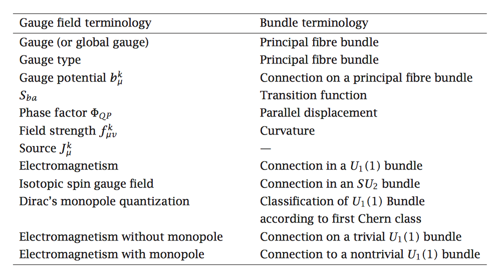